Excel is a powerful tool with numerous functions that allow users to perform a wide range of calculations and data analysis tasks. One of the most useful functions, particularly when working with numerical data, is the RANK function. This function allows you to determine the rank of a number relative to other numbers in a data set. Whether you’re comparing sales figures, grades, or any other set of numbers, the RANK function can help you quickly find where each value stands.
What is the RANK Function?
The RANK function in Excel returns the rank of a number in a list of numbers. Its primary purpose is to assign a rank to a number by comparing it to other numbers in the same list.
Syntax of the RANK Function
The syntax for the RANK function is straightforward:
=RANK(number, ref, [order])- number: This is the number you want to rank.
- ref: The range of numbers in which the “number” will be ranked.
- order (optional): This argument defines how to rank the numbers:
- 0 (or omitted): Ranks numbers in descending order (from highest to lowest).
- 1: Ranks numbers in ascending order (from lowest to highest).
Example of the RANK Function in Use
Let’s say you have a list of exam scores, and you want to find out how each student ranked in the class. Here’s an example dataset:
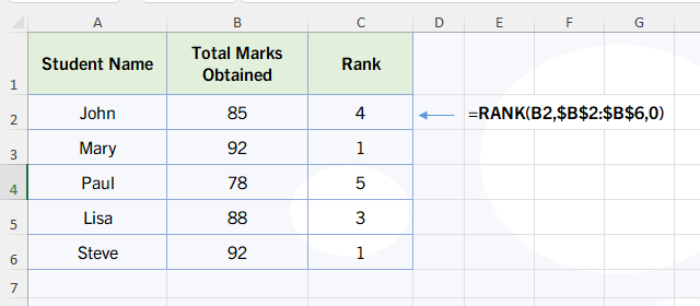
To find out how each student’s score ranks, you can use the RANK function. Use dollar symbols in B2:B6 range because it should remain constant when we drag the formula down for other students.
=RANK(B2, $B$2:$B$6, 0)This formula would assign a rank to the score in cell B2 (John’s score) compared to the scores in cells B2:B6.
The result would be 4 because John has the 4th score.
Handling Tied Ranks
In cases where two or more numbers in the list are the same, the RANK function will assign the same rank to each of those numbers. However, this can leave a gap in the ranking sequence. For example, in the dataset above, both Mary and Steve have a score of 92. Excel will assign both of them a rank of 1, and the next highest score will be ranked 3, skipping rank 2.
If you prefer to resolve ties differently, such as assigning unique ranks to tied values, you will need to use additional formulas or approaches, such as combining the RANK function with other functions like COUNTIF.
=RANK(B2,$B$2:$B$6,0)+(COUNTIF($B$2:B2,B2)-1)Use above formula in case you need to ignore the tied values.
Practical Applications of the RANK Function
The RANK function is widely used in various contexts, such as:
- Sales Analysis: Ranking sales figures for a team of salespeople to see who is performing the best.
- Academic Grading: Ranking students’ exam scores to determine the top performers.
- Competitions: Assigning rankings to competitors based on their scores or times.
- Financial Analysis: Ranking stocks or investment returns based on performance.
Alternative Functions: RANK.AVG and RANK.EQ
In Excel 2010 and later versions, the RANK function has two alternatives:
- RANK.EQ: Works the same way as the RANK function and is essentially an updated version of it.
- RANK.AVG: This function assigns tied values the average of their ranks. So, instead of skipping ranks, it smooths out the ranking.
For example, if two students share the top score in a class of five, their ranks will be averaged. Instead of both students being ranked 1 and the next ranked 3, both students will be ranked 1.5.
The syntax for these functions is the same:
=RANK.EQ(number, ref, [order])
=RANK.AVG(number, ref, [order])
Conclusion
The RANK function is an essential tool in Excel for quickly determining the position of a value within a set of numbers. Whether you’re ranking scores, sales figures, or any other numerical data, mastering this function will enhance your ability to analyze data effectively. If you frequently work with large datasets, consider using RANK.AVG or RANK.EQ for more refined results, especially when handling ties.
By understanding how to use the RANK function, you can add a powerful tool to your Excel skillset and make your data analysis more efficient and insightful.