How to Create Inventory Management Sheet in Excel

Overview

Managing inventory effectively is crucial for businesses to track stock levels, purchase and sakes. Excel is an excellent tool for creating a customized inventory management system. In this guide, we’ll walk you through the process of creating a functional inventory management sheet in Excel, from setting up your columns to using formulas to track stock levels and sales.

Steps of Creating Inventory Management Sheet

Follow these steps to create the inventory management sheet.

Step 1: Write the Title of the Sheet

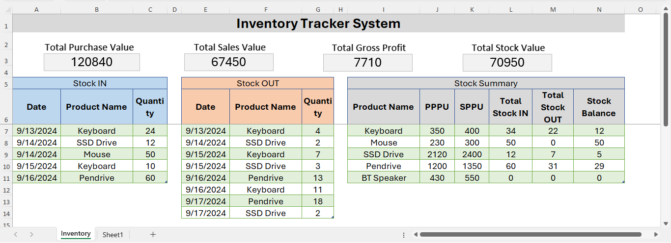
In an Excel sheet, select A1 to N1 cell range, merge them and write the title of sheet i.e “Inventory Management Sheet”.

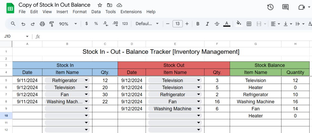
Step 2: Create Table for Stock IN, Stock OUT and Stock Summary

Stock IN (Purchase) Table

1. Select A5:C5 range and merge.
2. Write “Stock IN” in the merged cells.
3. Below it (Row number 6), write the column headers of Date, Product Name and Quantity.
4. Select the column headers and one row below it.
5. Press Ctrl + T in keyboard to create table.
6. In the create table dialog box, select my table has headers option and click on ok.

Stock OUT (Sales) Table

1. Select E5:G5 range and merge.
2. Write “Stock OUT” in the merged cells.
3. Beow it write the column headers of Date, Product Name and Quantity.
4. Select column headers and one row below it.
5. Press Ctrl + T in keyboard to create table.
6. Click on my table has headers option and click Ok.

Stock Summary Table

1. Select I5:N5 range and merge.
2. Write “Stock Summary” in the merged cells.
3. Beow it write the column headers of Product Name, PPPU, SPPU, Total Stock IN, Total Stock OUT and Stock Balance.
4. Select column headers and one row below it.
5. Press Ctrl + T in keyboard to create table.
6. Click on my table has headers option and click Ok.

Step 3: Enter the Product Names, Price and Create Drop Down List to Select Products

In the Product Name column of Stock summary table, enter all the products that you have and their purchase price per unit and sellingprice per unt. Then, create drop down list in Product Name column of Stock IN and Stock OUT table. To create drop down list, follow below given steps.

1. Click on B7 cell.
2. Click on data tab, then data validation.
3. In the data validation dialog box, within setting tab, choose List in the Allow menu.
4. In Source, select the product name list that you created in the Stock Summary table.
5. Click on ok. This creates a product selection menu.

Follow the same step to create product selection menu in the F7 cell (for Stock Out table).

Step 4: Use formula to calculate the Total Stock IN, Total Stock OUT and Balance

To calculate Total Stock IN, use below given formula in the L7 cell.

=SUMIF(Table4[Product Name],[@[Product Name]],Table4[Quantity])

In above formula, Table4 refers to purchase table. Replace this with your table name.

To calculate Total Stock OUT, use below given formula in the M7 cell.

=SUMIF(Table5[Product Name],[@[Product Name]],Table5[Quantity])

In above formula, Table5 refers to Stock Out table. Replace this with your table name.

To calculate stock balance, use below formula in the N7 cell.

=[@[Total Stock IN]]-[@[Total Stock OUT]]

This formula is subtracting the Total Stock Out from Total Stock IN of the Stock summary table.

Step 5: Test the formula

Now, test whether the used formulas are working perfectly or not. For this input some transaction details in the Stock In and Stock Out table. Cross check the calculations manually for few products just to ensure that there is no error in the formula.

Step 6: Create textboxes to display the overall status of inventory

Above the tables, create 4 textbox to display total purchase value, total sales value, total gross profit and total stock value.

To insert text box, click on Insert tab, Text, then Textbox.

Step 7: Calculate the values of Purchase, Sales, Gross Profit and Total Stock.

In the cells beside every textbox, calculate the value of purchase, sales, gross profit and stock. Later, we will link these values to the textbox.

Use below given formulas to calculate the required values.

Formula for Total Purchase

=SUMPRODUCT(Table6[Total Stock IN],Table6[PPPU])

Formula for Total Sales

=SUMPRODUCT(Table6[Total Stock OUT],Table6[SPPU])

Formula for Gross Profit

=SUMPRODUCT(Table6[Total Stock OUT],Table6[SPPU])-SUMPRODUCT(Table6[Total Stock OUT],Table6[PPPU])

Formula for Stock Value

=SUMPRODUCT(Table6[Stock Balance],Table6[SPPU])

Step 8: Link Calculated Values to Textbox

To link the values to textbox, follow these steps.

1. Click on outside border of textbox.
2. Click on formula bar.
3. Press = symbol, then click on the value calculated cell.
4. Press enter.

This will show the value inside text box. Use the formatting options to make the font size bigger and to change the alignment of text.

For every textbox, repeat the same steps.

After completing all these steps, you will be able to create this inventory management sheet in Excel. For more clarity of the steps, watch the video tutorial given below.

File Download

If you want the sample workbook file to practice this, download it form the button below.

Video Tutorial

Watch the video tutorial on step-by-step guide of making this from below.