The XLOOKUP function in Excel is one of the most powerful tools for searching and retrieving data. Introduced in 2019, XLOOKUP is an upgrade to the VLOOKUP and HLOOKUP functions, providing more flexibility and functionality. Unlike VLOOKUP, which has limitations such as requiring a column index and being restricted to left-to-right searches, XLOOKUP can search in both directions (vertical or horizontal), return arrays, and handle missing values gracefully.
In this article, we will explore the XLOOKUP function, its syntax, and provide multiple real-world examples to help you understand how to utilize this versatile tool.
What is XLOOKUP?
The XLOOKUP function searches a range or an array and returns a value that matches the criteria you provide. It works for both vertical and horizontal lookups and is more dynamic compared to older functions like VLOOKUP and HLOOKUP.
Syntax of XLOOKUP
=XLOOKUP(lookup_value, lookup_array, return_array, [if_not_found], [match_mode], [search_mode])Breakdown of the arguments:
- lookup_value: The value you want to search for.
- lookup_array: The array or range where you’re searching for the lookup_value.
- return_array: The range from which to return the result once a match is found.
- [if_not_found] (optional): The value to return if no match is found. If omitted, XLOOKUP returns an error if no match is found.
- [match_mode] (optional): Determines the type of match:
- 0: Exact match (default).
- -1: Exact match or next smaller item.
- 1: Exact match or next larger item.
- 2: Wildcard match.
- [search_mode] (optional): Specifies the search direction:
- 1: Search from the first to the last item (default).
- -1: Search from the last to the first item (reverse search).
- 2: Binary search in ascending order (data must be sorted).
- -2: Binary search in descending order (data must be sorted).
Example 1: Basic Vertical Lookup
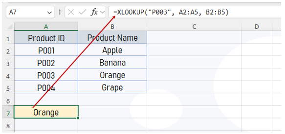
In this example, we have a table listing product IDs and their corresponding names. We will use XLOOKUP to find the product name based on its ID.
Data
Requirement
Find the product name for Product ID P003.
Formula
=XLOOKUP("P003", A2:A5, B2:B5)Result
The formula will return Orange because it matches the Product ID “P003” in column A and retrieves the corresponding value from column B.
Example 2: Reverse Lookup (Right to Left)
Unlike VLOOKUP, XLOOKUP can search for values in reverse. This means you can search in the return column and pull data from the lookup column.
Data

Requirement
Find the Product ID for the product name “Grape.”
Formula
=XLOOKUP("Grape", B2:B5, A2:A5)Result
The formula will return P004 as it looks for “Grape” in column B and returns the corresponding value from column A.
Example 3: Using the [if_not_found] Argument
XLOOKUP provides an option to handle missing data gracefully by using the [if_not_found] argument.
Data

Requirement
Let’s search for Employee ID E005. Since it doesn’t exist in the data, we want to display a message saying “Employee Not Found.”
Formula
=XLOOKUP("E005", A2:A5, B2:B5, "Employee Not Found")Result
Since “E005” is not found, the formula will return “Employee Not Found” instead of an error.
Example 4: Horizontal Lookup
XLOOKUP can also perform horizontal lookups. Suppose we have sales data for different products across various months.
Data

Requirement
We want to find the sales for Product B in March.
Formula
=XLOOKUP("Mar", B1:E1, B3:E3)Result
The formula will return 500, as it looks for “Mar” in the row B1:E1 and returns the corresponding value from the second row (Product B).
Example 5: Approximate Match
In some cases, you may want to return the closest match if an exact match doesn’t exist. For example, you want to find the price bracket for a specific salary.
Data

Requirement
We want to find the bonus for an employee with a salary of 45000. Since 45000 isn’t listed, we will return the next smaller salary’s bonus.
Formula
=XLOOKUP(45000, A2:A5, B2:B5, , -1)Result
The formula will return 700, as 40000 is the closest lower salary to 45000, and its bonus is 700.
Example 6: Wildcard Match
XLOOKUP can also perform searches using wildcards, allowing you to search for partial matches. This is particularly useful when dealing with text data.
Data
Requirement
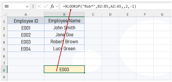
We want to find the employee with a last name that starts with “Rob”
Formula
=XLOOKUP("Rob*", B2:B5, A2:A5, , 2)Result
The formula will return E003, as “Rob*” matches “Robert Brown.”
Conclusion
The XLOOKUP function is a versatile and powerful tool for both vertical and horizontal lookups, reverse searches, and much more. Its ability to handle errors gracefully, find approximate matches, and use wildcards makes it a must-know function for any Excel user.
Whether you’re searching for a specific value, handling missing data, or performing complex lookups, XLOOKUP is the go-to function that will simplify your work and enhance your productivity.
So, dive into XLOOKUP and make your data searching more efficient!

