In this tutorial, we will learn how to freeze top row or any other n number of rows in Microsoft Excel. This is useful when we have big data and when we scroll down the data, the top row or few rows in the top row should be visible. Specially the headers or the title of columns should be visible to easily read the data.
See in below example, when we scroll the data down, the column headers hides. This makes difficulty in reading the data. So the need of row freezing emerge.
Steps of Freezing Rows in Excel
For freezing rows, let’s divide this into two instances.
- Freezing the Top Row
- Freezing the N number of Rows
Freezing the Top Row
If your data has the header in first row (row number 1), follow these steps.
- Click on View Tab.
- Click on “Freeze Panes.”
- Click on “Freeze Top Row.”

Now when you scroll down, the column headers are visible.
Freezing N Number of Rows
If your data header occupies more than one row, then the process is little different. Follow these steps for this.
- Click on the cell above which you want to freeze data. For example, if you want to freeze till row number 3, select the A4 cell. If you want to freeze 5 rows at top and 2 columns at left, select the C6 cell.
- Click on View Tab.
- Click on “Freeze Panes” tool, then “Freeze Panes” again.
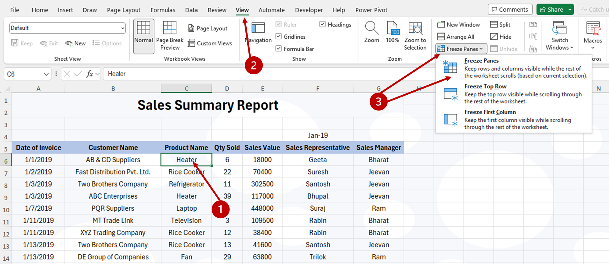
Now when scroll down and right, 5 rows at top and 2 columns at left remains freeze.