In this tutorial we are going to learn how to automatically highlight the active cell’s row in Excel. This we will do by using the conditional formatting tool and a small line of macro code.
See below image illustration where the active row is getting highlighted automatically.

Doing this basically involves three parts.
- Setting up Conditional Formatting Rule
- Writing VBA Code
- Save workbook as Macro Enabled
Setting Up Conditional Formatting Rule for Auto Highlighting Active Cell Row
Let’s start with the process.
Step1. Get the data ready. You can download the sample data from end of this post.
Step2. Select the data range where you want to apply the automatic highlighting.
Step 3. Click on “Home” tab.
Step 4. Click on “Conditional Formatting”.
Step 5. Click on “New Rule”.

Step 6. In the “New Formatting Rule” dialog box, click on “use a formula to determine which cell to format”.
Step 7. In the Formula bar write =Cell(“Row”)=Row()
Step 8. Click on “Format” button. (this will open “Format Cell” Dialog box.
Step 9. Click On “Fill” tab.
Step 10. Choose the color that you want for highlighting.
Step 11. Click on “Ok” button of both dialog box.

Now you have finished setting up the conditional formatting rule. The highlight applies to the active row. But when you switch to other cell, this doesn’t update in real time. For this we have to use VBA code to auto update this.
Write the VBA Code
Step 1. Click on “Developer” Tab.
Step 2. Click on “Visual Basics”.

Step 3. Visual basic for applications window opens. Then Double click on sheet name (where you have the data for highlight).
Step 4. Click on the Dropdown.
Step 5. Choose “Worksheet”

Step 6. Write VBA Code at mid “application.screenupdating=true”
Step 7. Close the VBA Editor Window

Done. Now when you select different cells, the selected cell’s row will get highlighted automatically.
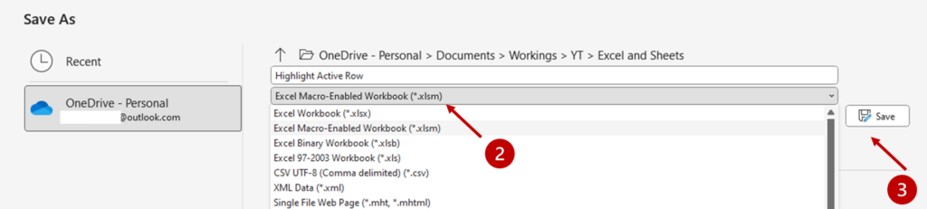
Save the workbook as Macro Enabled Workbook
Now to use this auto highlight next time when you open the file, you need to save the workbook as “Macro Enabled File”.
Follow these steps.
Step 1. Click on “File” tab then “Save As”.

Step 2. In the file type choose “Excel Macro Enabled Workbook”
Step 3. Click on “Save” Button by choosing your desired location.
All done. Now You can use your file with the feature of Automatic Highlight of Active Row.
Note: If you want to remove the automatic highlighting, select your whole data > Home Tab > Conditional Formatting > Clear Rules > Clear Rules from the Selected Cells. Click on Visual Basics and delete the code. You can also save the file as normal workbook (no macro enabled), then the code gets auto removed.
Download the workbook file for practice.


The sample file does not even work. What’s wrong? I’m using Excel 2021 for Win 10 Pro on my PC.
Is this only for Office 365 versions of Excel?
There was an issue with sample file, now it has been updated and works perfectly.