Auto Highlight Row Based on Value in a Cell of Column in Excel

In this article, you will learn how to automatically highlight the entire row of data based on value in a column in Microsoft Excel.

Table of Contents

1. Use and Importance
2. Example
3. Steps of Auto Highlighting Row
4. Removing the Auto Highlight
5. Practice Workbook Download
6. Video Tutorial

1. Use and Importance

Automatically highlighting rows based on cell values in Excel is crucial for enhancing data visibility, simplifying decision-making, and improving efficiency. It helps quickly identify important data, detect errors, and track performance by providing real-time visual cues in large datasets. This feature makes data more readable, supports monitoring tasks like inventory levels or sales targets, and offers flexibility in applying custom rules to suit various needs. Ultimately, it streamlines data management and reporting, ensuring that key information stands out for timely action.

2. Example

For example, you have an invoice and payment tracker format in Excel sheet where you have details of the invoice and their payments. In the last column, there is status of invoice. Requirement is to highlight the rows if the status of invoice is marked as “Paid”. See below example for more clarity.

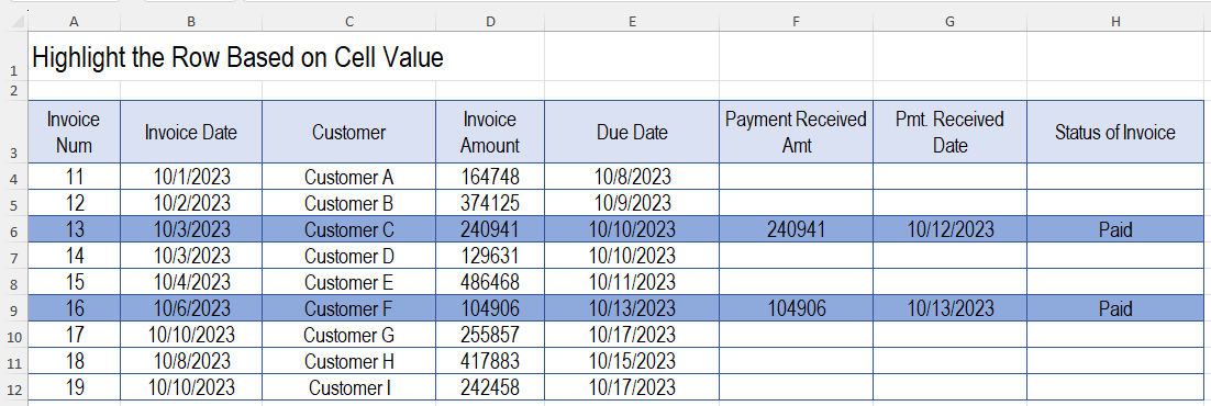
In the example, while there is status invoice is “Paid”, row gets auto highlighted with blue color.

3. Steps of Auto Highlight Row

Follow these steps to auto highlight row based on cell value.

1. Prepare the data: First, you should have a data where you require to highlight some special rows to make them unique. In this example, by highlighting the “Paid” invoices, it makes it distinct and easy to figure out the paid invoices. Another example can be a task tracker format where you need to auto highlight the completed tasks.
2. Select your entire data excluding the column headers.
3. Click on Home tab > Conditional Formatting > New Rule > Use a formula to determine which cell to format.
4. In the formula box write this formula =$H4=”Paid”. [In this formula H is the column where your conditional value is. 4 is the first row number just below the column headers.]
5. Click on Format button.
6. Click on Fill tab. Choose the color that you want for highlighting and click on Ok.

After completing these steps, the rows with the value “Paid” in H column will be auto highlighted. IF you change the value to different one, color highlight will remove automatically. And, when you mark it as “Paid”, highlighting appears.

4. Removing the Auto Highlight

To remove the auto highlight, follow these steps.

1. Select the entire data.
2. Click on Home Tab > Conditional Formatting > Clear Rule > Clear Rule from the Selected Cells.

5. Practice Workbook File Download

If you want to practice doing this, download the sample data file from below.

6. Video Tutorial

For the step-by-step guideline on how to auto highlight row based on value in a column, watch video tutorial given below.