This article covers the guideline on how to calculate SUM based on selection of drop-down list in Google Sheets.
Importance
Calculating the SUM based on a selection of dropdown list in Google Sheets is a powerful feature for dynamic data analysis. It allows users to easily filter and summarize data by specific categories, such as departments, products, or dates, simply by selecting an option from a dropdown menu. This not only saves time but also enhances decision-making by providing instant insights tailored to the selected criteria. It’s especially useful in dashboards and reports, where interactivity and clarity are essential for understanding trends and making informed choices.
Watch Tutorial on How to Make Drop Down List in Google Sheets: https://youtu.be/NCImWB4c3wI
Practical Examples
Example 1
You have a data of personal expenses where the expenses category is repeating multiple times. You want to calculate the total expenses for the category item you choose from a drop-down list.
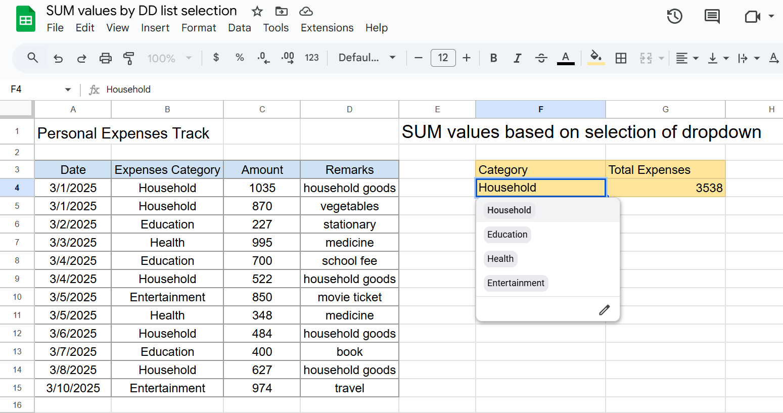
In the above example, column A to D has the details of expenses, where the expenses category items like Household, Education etc. are repeating on multiple dates. In the F4 cell, there is a drop-down selection list and based on the category item selected, total expenses should be calculated in the G4 cell. In this case, we can use the SUMIF function. Because SUMIF function in Google Sheets calculates the sum of numbers based on a condition.
Formula
To calculate SUM by selection of drop-down list, use below formula in the G4 cell.
=SUMIF(B4:B15,F4,C4:C15)This formula will find the expenses category selected in F4 cell in the B4:B15 range and add the corresponding amounts and return the total in G4 cell.
Example 2
You have a sales data for different products for different months. You want to calculate the total sales quantity for different months for a specific product that is selected form a drop-down list.

In above example, column A to E has the details of quantity sold for different products which are sold in different stores in different months. Requirement is to calculate the total quantity sold in different months for the product that is selected from the drop-down list in the G4 cell. In this case, we can again use the SUMIF function with some addition in the formula.
Formula
To calculate sum by selection of drop-down list, use below given formula in the H4 cell, then copy the same formula for I4 and J4 cell.
=SUMIF($B$4:$B$15,$G4,C4:C15)In the formula, you have to lock B4:B15 range and G4 range by using the dollar symbol($), because when you copy the formula for other cells, these range and cell should remain constant.
Google Sheets Link
If you want to practice this in above mentioned data, open the google sheets by clicking on below button. It will ask you to make a copy of the document. Click on “Make a Copy” button.


How do you do this but needing to calculate by multiple categories? Do you need ‘[ ]’ or use ‘ ( )’ and ‘&’?
for multiple categories, use the SUMIFS function. for SUMIFS function guide, watch this tutorial: https://youtu.be/9mBLbzV2Di0