How to Automatically Highlight Active Cell’s Row Column in Google Sheets

In this tutorial, we will learn how to automatically highlight the active cell’s row column in Google Sheets. Note that this will remove the previously highlighted colors from the sheet. If your sheet has important colors applied, which should not be removed, do not apply this.

This basically has below steps.

1. Get the Apps Script code
2. Install the code
3. Save and run the code
4. Change the Color for Highlighting

Get The Apps Script

First of all you need to have an Apps Script. The script you can copy from the end of this tutorial.

Install the Code

To install the script in your Google Sheets document, follow these steps.

Step 1. Copy the script from downloaded notepad file.

Step 2. Click on “Extensions” tab of Google Sheets then click on “Apps Script”.

Step 3. Click on + button beside “Files” then click on “Script”.

Step 4. A script page with the name “untitled” gets created. Change the name or you can take the default name too.

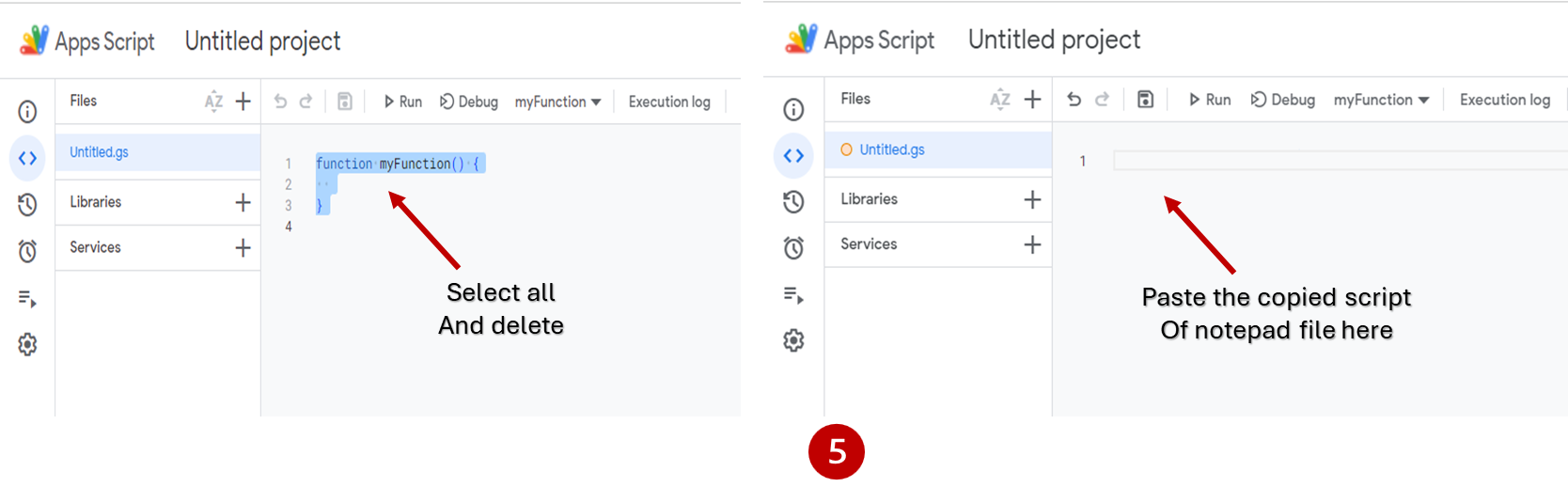
Step 5. Click in the blank area of script page. Select all the script given there and delete them. Then, paste the copied script from notepad.

Step 6. Change the actual name of your sheet in the script.

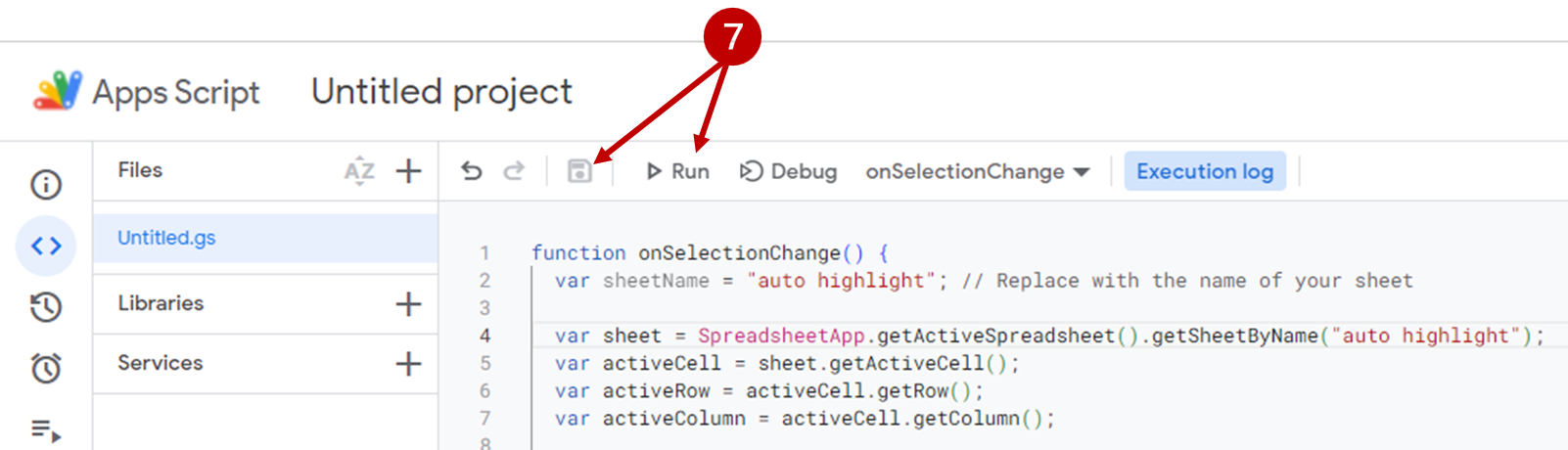
Step 7. Save the script and run it. While running the code for the first time, it will ask you for some permission.

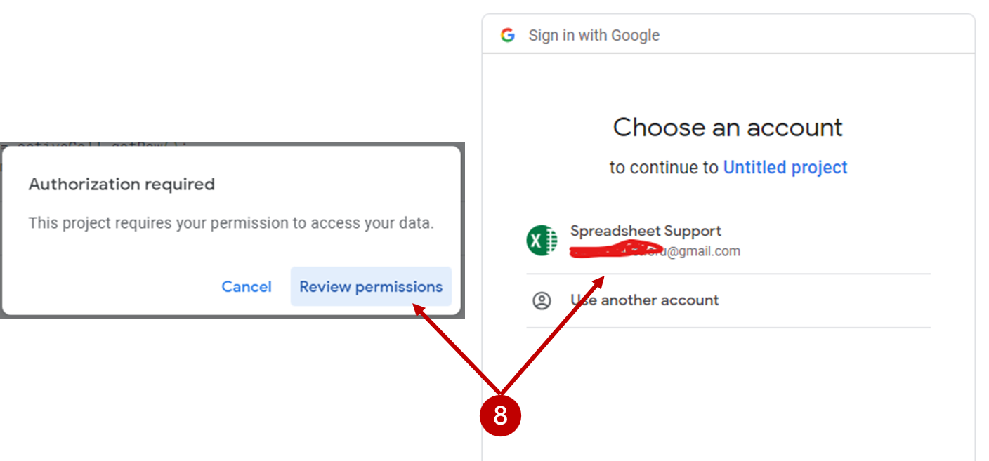
Step 8. Click on “Review Permission”, then click on your Google Account.

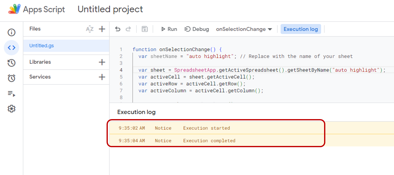
Step 9. Click on “Advanced” and then click on “Go to untitled project” then click on “Allow” button. You will see “execution started” and “execution completed” in the execution log. It means the script has no error.

Step 10. Go to your google sheets documents and click on reload button of the browser or app window.

Now the active cell’s row and column has the highlight.

Change The Color of Highlight

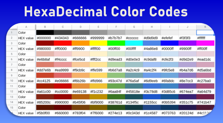
If you want to change the color for highlighting, you can set up a different color for row and column. For this locate the color used in the script. Replace it by color name or hexadecimal color code value.

You can find the color and their hexadecimal code in below image. After setting up the color, save the script and reload your document. New color will now apply.

Apps Script

Copy the script from below.

function onSelectionChange() {
  var sheetName = "auto highlight row"; // Replace with the name of your sheet
  
  var sheet = SpreadsheetApp.getActiveSpreadsheet().getSheetByName("auto highlight row");
  var activeCell = sheet.getActiveCell();
  var activeRow = activeCell.getRow();
  var activeColumn = activeCell.getColumn();
  
  var range = sheet.getDataRange();
  var numRows = range.getNumRows();
  var numColumns = range.getNumColumns();
  
  var topRow = sheet.getFrozenRows() + 1; // Skip frozen rows (if any)
  
  var rowRange = sheet.getRange(topRow, 1, numRows - topRow + 1, numColumns);
  var columnRange = sheet.getRange(1, activeColumn, numRows, numColumns - activeColumn + 1);
  
  rowRange.setBackground(null); // Reset row background
  columnRange.setBackground(null); // Reset column background
  
  var rowBackground = "lightblue"; // Replace with your desired row background color
  var columnBackground = "lightgreen"; // Replace with your desired column background color
  
  sheet.getRange(activeRow, 1, 1, numColumns).setBackground(rowBackground); // Highlight row
  sheet.getRange(1, activeColumn, numRows, 1).setBackground(columnBackground); // Highlight column
}

What If You want to Auto Highlight the Row Only

In case you want to auto highlight the active row only, please use below given script.

function onSelectionChange() {
  var SheetName = "data_source"; // replace with the name of your target sheet
  var sheet = SpreadsheetApp.getActiveSpreadsheet().getSheetByName("data_source");

  if (!sheet) {
    Logger.log("Sheet not found");
    return;    
  }

  var activeRange = sheet.getActiveRange();
  var activeRow = activeRange.getRow();

  // clear existing row highlight
  var lastColumn = sheet.getLastColumn();
  var lastRow = sheet.getLastRow();
  sheet.getRange(2, 1, lastRow - 1, lastColumn).setBackground(null); // start from row 2, skipping top row

  // highlight the active row
  sheet.getRange(activeRow, 1, 1, lastColumn).setBackground('yellow');  
}