In this tutorial you will learn how to make drop-down menu list in Microsoft Excel.
Drop-Down list is useful when we have to select from multiple values to be entered in a cell. This also helps on easy and error free entry of data.
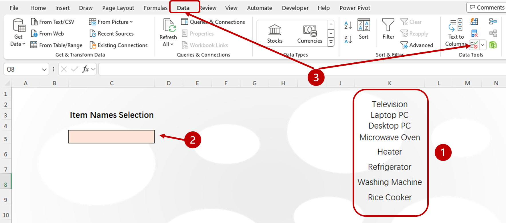
See below illustration for what is drop-down menu in excel.

In the example above, you can choose from multiple values to input in a cell. This is called the drop-down menu in Excel.
Process of Making Drop Down List
Process of making drop down menu is same for any type of values. Here we will make the drop-down menu for Item Names (see column F in above example). Follow these steps to make drop down menu in Excel.
Step 1. Prepare the list of items to show in drop – down menu.
Step 2. Click on the cell where you want to make the drop-down list.
Step 3. Click on “Data” Tab then “Data Validation.” This will Open Data Validation dialog box.
Step 4. Click on “Setting” tab, activate drop down menu, then click on “List”.
Step 5. Click in the source bar, then select the item name list you have prepared in step 1.
Step 6. Click on “Ok”.

Now you will see a menu expansion button at the right side of the cell (for this you need to click on the cell). Hover the mouse pointer on the button and click. You will have a item selection list there. Click and choose the item that you need to place in the cell.

More on Data Validation
Data validation is one of the very useful tool in Excel. It has great use for data entry and analysis job. Creating drop down menu is only one branch of data validation. If you want to explore full knowledge on data validation topic, please watch the YouTube video tutorial from the link below.


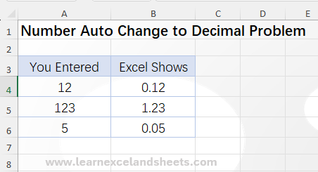


Pingback: Number Auto Change to Decimal in Excel: Learn How to Solve - Learn Excel and Sheets