In this article, you will learn 10 essential Excel formulas for beginners that is very useful for the beginners in learning Microsoft Excel.
Formulas in Excel are the expressions that performs different kind of calculations. There are more than 400 pre-defined formulas in Excel which are generally known as functions. Here, we are looking into 10 functions that are important specially for the beginners in learning Excel.
SUM Function
SUM function in Excel is used for adding the numbers in cells or ranges. Formula syntax is =SUM(number1,[number2],…)
In number 1 and number 2 parameters, you can put a cell address, range or the numbers themselves.
Example
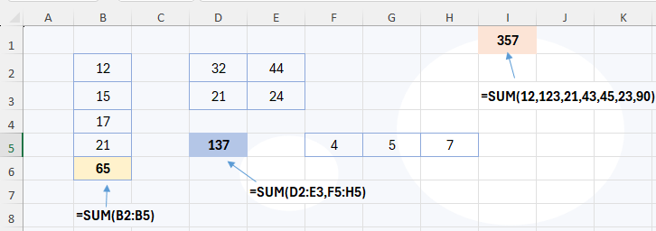
In the example above, SUM function is used to calculate the total of different numbers. See below table for more clarity.
| Formula | Description | Result |
| =SUM(B2:B5) | Adds the numbers in B2 to B5 range. | 65 |
| =SUM(D2:E3,F5:H5) | Adds the numbers in two ranges. Separate each range by a comma. | 137 |
| =SUM(12,123,21,43,45,23,90) | Adds all the absolute numbers provided to the formula. Separate each number by comma. | 357 |
COUNT Function
COUNT function counts the number of cells that contains the numeric values only. Formula syntax of COUNT function is =COUNT(value1,[value2]…)
In the value1, value2 parameters, we have to put the cell range or absolute values. If there are more than one range, each range should be separated by comma.
Example
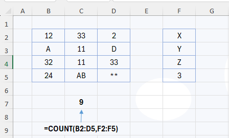
In the example, count function has counted the number of cells that contains only the numeric values. In B2:D5 and F2:F5 range, there are total 16 cells filled with some type of data. Out of them, 9 cells have the numeric values, and the result of the formula is 9.
COUNTA Function
COUNTA function counts the number of cells that has any type of value. In other words, COUNTA counts all non-blank cells in a range. Formula syntax is =COUNTA(value1, [value2], …)
In the value1, value2 parameters, we have to put the cell range or absolute values. If there are more than one range, each range should be separated by comma.
Example
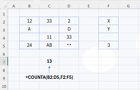
In the example, COUNTA function counted all the non-blank cells in the range. Out of these 16 cells, 13 cell are non-blank. Hence the result of COUNTA function is 13.
COUNTBLANK Function
COUNTBLANK function calculates the number of blank cells in a range. Formula syntax is =COUNTBLANK(range).
Unlike aforementioned functions, we cannot use multiple ranges in this function. In below example, there are two separate ranges. So, the COUNTBLANK is used two times.
Example
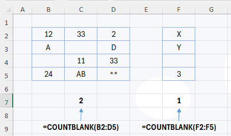
In the first range, there are 2 empty cells. Result is calculated as 2. Similarly, in second range, result is 1.
AVERAGE Function
AVERAGE function in Excel calculates the arithmetic mean value of the numbers. Formula syntax is =AVERAGE(number1, [number2], …). In the number1, number2 parameters, we can put an array, numbers, named range or reference.
Example
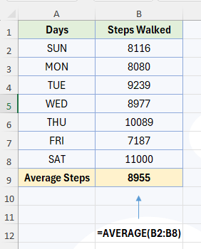
In the example, the average steps walked in a week is calculated by using the average function.
MIN and MAX Function
MIN and MAX function in Excel are used for finding the smallest and largest number from a set of numbers. Formula syntax is =MIN(number1, [number2], …)
Example
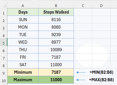
In the example, the smallest and largest number of steps walked is calculated as 7187 and 11000 by using the MIN and MAX functions.
RANK Function
RANK function is used for calculating the rank of a number in a list of numbers. Formula syntax is =RANK(number, reference, [order]).
Example

In the example, rank of mark obtained is calculated using the rank function. In the order parameter of formula, 0 represents descending order. Which is the highest to lowest order and the highest number will get first rank and lowest will get last rank. On the other hand, 1 represents ascending order in which lowest value will get the first rank. So, here in case of marks obtained in exam, we have to take highest number in first rank. So, 0 is taken in the order. Out of all students, name 6 has got the highest score that is 798 and has got the first rank.
IF Function
IF function in Excel checks whether a condition is met, if result is TRUE, returns one value. If result is FALSE, returns another value. The formula syntax is, =IF(logical_test, [value_if_true],[value_if_false]).
Example
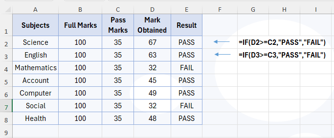
In the example, in logical test parameter of the formula, D2>=C2 is checking whether the mark obtained is greater than or equal to pass mark. If this logic is true, then PASS is displayed. IF this logic is not true, then “FAIL” is displayed. In value if true and value if false parameters, if we are putting the text, it should be enclosed with double quotations (” text”). If we are putting number or formula, double quotation should not be used.
TRIM Function
TRIM function in Excel is used to remove all spaces from a text string except a single space between words. This is very useful function for data cleaning. It removes all unwanted space that may occur due to typo. Formula syntax is =TRIM(text).
Example
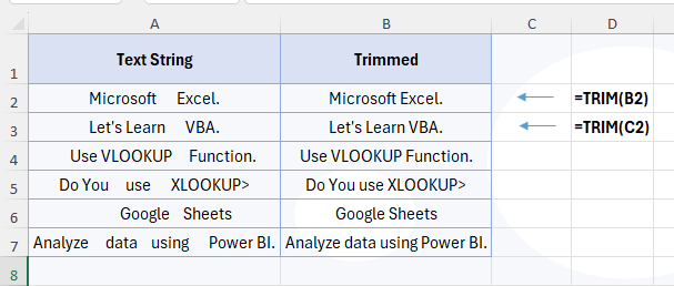
In the example, in column A, there are text strings which has unwanted or more than one space between words. Some string has multiple spaces before the starting letter too. In this case, TRIM function is used to clean the data. In column B, new text string is given by removing all unwanted spaces.
ROUND Function
ROUND function is used to round a number to specified number of digits. Formula syntax is =ROUND(number, num_digits).
Example
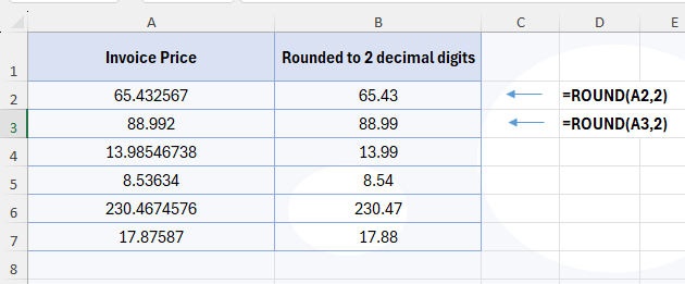
In the example, in column A, there are invoice price that has multiple digits after decimal. Requirement is to round them with digits after decimal. In column B, ROUND function is used for rounding. In num_digits parameter, you can put any number according to your requirement.
Conclusion
Familiarizing yourself with these will help you navigate Excel efficiently and get the most out of it for everyday tasks. There are many other functions in Excel that you should learn to expertise your skill in Excel. For other functions, tools, tips, tricks and tutorials in Excel, navigate to the menu bar above. Thank you for reading this article.
Workbook Download
If you want to download the practice file to practice these functions, get it from below.


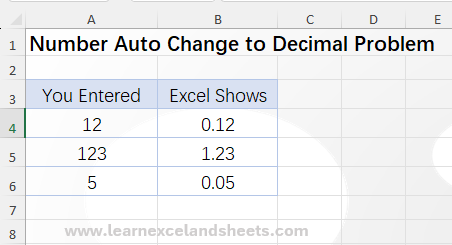


Pingback: Number Auto Change to Decimal in Excel: Learn How to Solve - Learn Excel and Sheets